This is something that I should have posted a long time ago, but didn’t come across suitable data until now.
To understand the distribution, we need to start with a frequency distribution. Look at the following image. If we have items of certain values, one could plot a graph showing how many times (frequency) an item of a given value appears (first row in Fig. 1). If we connect the datapoints (red crosses) we get a frequency distribution curve (second row in Fig. 1). Sometimes we have a frequency distribution curve as in the third row of Fig. 1, where the vertical axis is still the number of times an item appears and the horizontal axis is the value of the item being considered. A frequency distribution curve as in the third row in Fig. 1 is known as a normal or Gaussian distribution. It is also referred to as the bell curve.
Fig. 1. Some frequency distributions.
If one has a normal distribution, one can easily calculate the proportion of the distribution that is above or below a certain value or between two values. I used an online calculator to come up with the following two examples, and you should play with it, too.
Fig. 2. In the left curve, the proportion of the distribution that lies over a value of 1.5 is 0.066807 or 6.6807%. In the right curve, the proportion of the distribution that lies below a value of -0.5 is 0.308538 or 30.8538%.
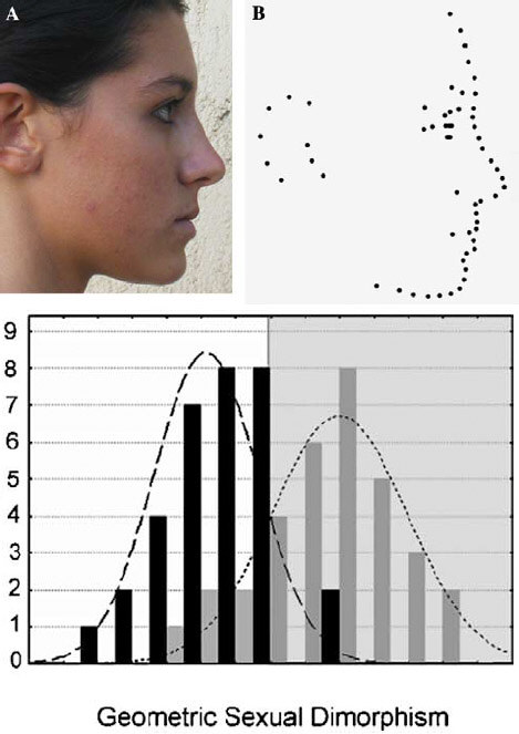
Now let us look at the data of Valenzano et al. (Fig. 3).(1, pdf) In the image below the first row shows the landmarks used to assess face shape. Each face can be represented by a point in shape-space that describes the set of the positions of all landmarks defining the face. One can compute the position of the average male and average female faces. The axis that joins these averages is the axis of sexual dimorphism. The geometric sexual dimorphism of each face is its position on this axis. Hence, one can plot a frequency distribution curve with the value on the horizontal axis being the geometric sexual dimorphism (Fig. 3 second row).
Fig. 3. First row shows landmarks used to assess face shape. Second row shows frequency distribution curve (number of faces lying at various positions of the sexual dimorphism axis); black bars represent males, grey bars represent females. The male frequency distribution curve is dashed and the female frequency distribution curve is dotted.
In the image below, one can observe in the graph on the left the proportion of men whose faces cannot be distinguished from women (shaded red) and the proportion of women whose faces cannot be distinguished from men (shaded green). A greater proportion of women cannot be distinguished from men compared to the proportion of men who cannot be distinguished from women. Use the calculator mentioned in the context of Fig. 2 to obtain a rough idea of what these proportions are. The image on the right is more interesting. It shows that the proportion of women more feminine than the most effeminate men is much greater (shaded green) than the proportion of men more masculine than the most masculine women (shaded red), and also that only a minority of women have faces more feminine than the most effeminate men.
Fig. 4. Proportion of faces that cannot be assigned to a sex (left) and proportion of faces that exceed extremes for the opposite sex.
The authors didn’t have a random sample, and the sample comprises of Italians, but I believe that the results shown above are roughly true for male-female differences. It doesn’t take much testosterone to make a woman look masculine but a lot of testosterone to make a man look masculine. Consider that effeminate men still have much higher testosterone levels than the most masculine women. Then there is the remarkable transformation that many women undergo as they age.
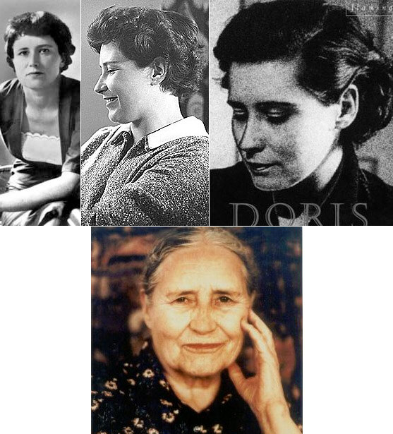
Consider the example of Doris Lessing below, the 2007 Nobel Laureate in literature. As a young woman, she wasn't feminine, but looked female. However, in old age her face has become that of a man's (no offense to her). I have seen too many similar examples to count.
Fig. 5. Doris Lessing
Another example is that of female bodybuilders. After they stop taking anabolic androgenic steroids, they don’t go back to where they came from; some masculinization remains, unlike men. There are also some analogies from sex-atypical behavior in children, presumably partially affected by the organizational effects of prenatal testosterone exposure. Sex-atypical behaviors are much more common among girls than boys. Again, it doesn’t take a lot of testosterone to masculinize women.
Hopefully after reading this people will stop accusing me of having a very broad concept of what is meant by masculinization in the looks of women.
References
- Valenzano, D. R., Mennucci, A., Tartarelli, G., and Cellerino, A., Shape analysis of female facial attractiveness, Vision Res, 46, 1282 (2006).
Comments
"However, in old age her face has become that of a man's (no offense to her)."
HAHAHAHAHAHAHAHAHAHA! I find the young Doris quite attractive, though that may be because I'm a heterosexual female. :/!!!
P.S. At least her hands don't look that manly! My grandma has horrible manly hands, ick!
Lessing, to me, looked like she already had a very strong jawline when she was younger.
In the picture where she's older, she just looks like an older lady to me, not masculine. The muscle and connective tissues in the face fall as we age, thus she doesn't have the same beauty when she's older.
Erik, concerning female body builders who stopped taking androgens, is there anything they can do to correct the masculinization that remains even after they have stopped taking the hormones? Does the reverse happen if a woman takes estrogen?