To start with, the apportionment of craniofacial diversity with respect to 57 linear measurements across 10 populations from William White Howells’ dataset(1) is considered below. The populations sampled are shown in Table 1.
Table 1. Populations studied.(2) |
|
South America |
Yauyos (110) |
China |
Anyang (42) |
Japan |
North Kyushu (91) |
Siberia |
Buriats (109) |
Europe |
Medieval Norse (110) |
Middle East |
Gizeh (111) |
Melanesia |
Tolai (83) |
East Africa |
Telta (83) |
South Africa |
!kung/San (90) |
West Africa |
Dogon (99) |
In molecular genetics, the apportionment of genetic diversity is often described in terms of Sewall Wright’s fixation index, FST, which is calculated by subtracting the average diversity within populations from the total diversity in the species and then dividing the result by the total diversity in the species. Therefore, if all the variation is within populations and none between, FST = 0. If all the variation is between populations and none within, FST = 1. Hence, higher FST values reveal greater differences between populations. FST values vary depending on the locus assessed. In animals, almost all genes are found in nuclear DNA, which is found in the nucleus of a cell. Overall FST values based on nuclear DNA are classified as suggesting the following extent of genetic differentiation between populations: 0-0.05, little differentiation; 0.05-0.15, moderate differentiation; 0.15-0.25, great differentiation; 0.25-plus, very great differentiation.(3) Overall FST based on nuclear DNA is about 0.15 for humans.
Roseman calculated QST values for 57 linear craniofacial measurements in the 10 populations shown in Table 1, and these values are shown in Table 2.(2) QST represents the same idea as FST, but is designated differently to distinguish it from FST. Table 2 shows that several craniofacial measurements vary very greatly across human populations. The overall QST value was 0.24, which borders on the very great. For any given set of facial measurements, a similar proportion of people across populations will match the set if QST = 0, but the problem is that QST values close to zero are attained for traits such as the length of the foramen magnum (a big hole in the bottom of the skull through which the spinal cord passes), which is a trait that is not relevant to a beauty contest. The facial measurements most relevant to a beauty contest -- such as distance between the eyes, forehead projection, nose height, jaw projection, etc. -- show very great differences across populations.
Table 2. QST values.(2) |
|||
Measurement |
QST |
Full measurement name (alphabetical order) |
|
AUB |
0.49 |
ASB, biasterionic breadth |
|
XCB |
0.47 |
AUB, biauricular breadth |
|
ZYB |
0.37 |
AVR, molar alveolus radius |
|
NLH |
0.37 |
BBH, basion-bregma height |
|
SIS |
0.36 |
BNL, basion-nasion length |
|
NDS |
0.35 |
BPL, basion-prosthion length |
|
WMH |
0.34 |
DKB, interorbital breadth |
|
WCB |
0.32 |
DKR, dacryon radius |
|
EKR |
0.31 |
DKS, dacryon subtense |
|
XFB |
0.31 |
EKB, biorbital breadth |
|
NPH |
0.30 |
EKR, ectoconchion radius |
|
ZOR |
0.28 |
FMB, bifrontal breadth |
|
SSR |
0.27 |
FMR, frontomalare radius |
|
VRR |
0.27 |
FOL, foramen magnum length |
|
FMR |
0.26 |
FRC, nasion-bregma chord |
|
PRR |
0.25 |
FRF, nasion-subtense fraction |
|
BBH |
0.25 |
FRS, nasion-bregma subtense |
|
ZMR |
0.25 |
GLS, glabella projection |
|
JUB |
0.25 |
GOL, glabella-occipital length |
|
ASB |
0.23 |
IML, malar length, inferior |
|
BPL |
0.23 |
JUB, bijugal breadth |
|
STB |
0.23 |
MAB, palate breadth |
|
DKR |
0.21 |
MDB, mastoid width |
|
NLB |
0.21 |
MDH, mastoid height |
|
NAR |
0.20 |
MLS, malar subtense |
|
GLS |
0.20 |
NAR, nasion radius |
|
SSS |
0.20 |
NAS, nasio-frontal subtense |
|
PAF |
0.19 |
NDS, naso-dacryal subtense |
|
AVR |
0.19 |
NLB, nasal breadth |
|
NAS |
0.18 |
NLH, nasal height |
|
IML |
0.18 |
NOL, nasio-occipital length |
|
XML |
0.18 |
NPH, nasion-prosthion height |
|
MAB |
0.18 |
OBB, orbit breadth |
|
OBH |
0.16 |
OBH, orbital height |
|
ZMB |
0.16 |
OCC, l-opisthion chord |
|
OCS |
0.15 |
OCF, l-subtense fraction |
|
BNL |
0.15 |
OCS, l-opisthion subtense |
|
EKB |
0.14 |
PAC, bregma-lambda chord |
|
GOL |
0.14 |
PAF, bregma-subtense fraction |
|
NOL |
0.14 |
PAS, bregma-lambda subtense |
|
DKS |
0.13 |
PRR, prosthion radius |
|
OBB |
0.13 |
SIS, simotic subtense |
|
FRS |
0.13 |
SOS, supraorbital projection |
|
FMB |
0.13 |
SSR, subspinale radius |
|
OCC |
0.12 |
SSS, bimaxillary subtense |
|
DKB |
0.11 |
STB, bistephanic breadth |
|
PAC |
0.11 |
VRR, vertex radius |
|
WNB |
0.10 |
WCB, minimum cranial breadth |
|
FRF |
0.09 |
WMH, cheek height |
|
SOS |
0.09 |
WNB, simotic chord |
|
MDH |
0.08 |
XCB, maximum cranial breadth |
|
MLS |
0.08 |
XFB, maximum frontal breadth |
|
FRC |
0.08 |
XML, malar length, maximum |
|
MDB |
0.08 |
ZMB, bimaxillary breadth |
|
PAS |
0.07 |
ZMR, zygomaxillare radius |
|
FOL |
0.05 |
ZOR, zygoorbitable radius |
|
OCF |
0.04 |
ZYB, bizygomatic breadth |
|
It could be pointed out that the measurements in Table 2 do not separate shape from size, but this separation is easily achieved by transforming the 57 linear measurements in Table 2 to shape variables (Mosimann shape variables), which is what Roseman and Weaver did to a more extensive set of William White Howells’ database (1,734 skulls from 6 regions; comprising of a total of 18 populations).(4)
The authors then extracted factors (principal components; PCs) underlying the covariation of the shape variables using principal components analysis (PCA). Three shape variables -- dacryon subtense, supraorbital projection, and glabella projection -- tended to dominate the first few PCs, and were therefore excluded from PCA. The respective variances explained by the first 8 principal components, starting from the first, were: 26.1%, 9.7%, 7.2%, 6.6%, 6.4%, 5.3%, 3.6% and 3.4%. The first 6 PCs were most relevant and together accounted for 61.3% of the variance. What the first six PCs correspond to is shown in Table 3 (bolded).
Table 3. Eigenvectors for first six principal components.(4) |
||||||
Measurement |
PC1 |
PC2 |
PC3 |
PC4 |
PC5 |
PC6 |
GOL: glabella-occipital length |
-0.03 |
0.02 |
-0.04 |
-0.04 |
0.05 |
0.02 |
NOL: nasio-occipital length |
-0.02 |
0.03 |
-0.05 |
-0.04 |
0.05 |
0.02 |
BNL: basion-nasion length |
-0.01 |
0.01 |
-0.02 |
0.03 |
-0.01 |
0.05 |
BBH: basion-bregma height |
-0.04 |
0.03 |
-0.03 |
-0.11 |
-0.01 |
-0.03 |
XCB: maximum cranial breadth |
-0.03 |
0.04 |
-0.05 |
-0.15 |
0.03 |
-0.04 |
XFB: maximum frontal breadth |
-0.03 |
0.07 |
-0.04 |
-0.16 |
0.00 |
-0.04 |
STB: bistephanic breadth |
-0.03 |
0.10 |
-0.06 |
-0.20 |
0.02 |
-0.05 |
ZYB: bizygomatic breadth |
-0.03 |
-0.01 |
0.01 |
-0.03 |
-0.01 |
-0.04 |
AUB: biauricular breadth |
-0.04 |
0.01 |
-0.02 |
-0.06 |
0.00 |
-0.03 |
WCB: minimum cranial breadth |
-0.04 |
0.01 |
-0.01 |
-0.09 |
0.00 |
-0.04 |
ASB: biasterionic breadth |
-0.03 |
0.02 |
-0.03 |
-0.09 |
0.07 |
-0.02 |
BPC: basion-prosthion length |
-0.04 |
0.01 |
0.02 |
0.05 |
-0.01 |
0.07 |
NPH: nasion-prosthion height |
-0.01 |
-0.07 |
-0.03 |
0.00 |
-0.02 |
-0.00 |
NLH: nasal height |
-0.00 |
-0.04 |
-0.05 |
-0.02 |
-0.03 |
0.00 |
OBH: orbital height |
-0.03 |
0.03 |
-0.10 |
-0.08 |
0.02 |
-0.01 |
OBB: orbit breadth |
-0.04 |
0.00 |
-0.04 |
-0.02 |
0.00 |
0.02 |
JUB: bijugal breadth |
-0.03 |
0.02 |
0.03 |
0.00 |
-0.02 |
-0.01 |
NLB: nasal breadth |
-0.02 |
0.09 |
0.01 |
0.01 |
-0.02 |
-0.00 |
MAB: palate breadth |
-0.04 |
-0.03 |
-0.00 |
-0.02 |
-0.01 |
-0.00 |
MDH: mastoid height |
0.02 |
-0.28 |
0.19 |
0.05 |
0.08 |
-0.48 |
MDB: mastoid width |
-0.02 |
-0.36 |
0.35 |
0.10 |
0.19 |
-0.42 |
ZMB: bimaxillary breadth |
-0.03 |
0.02 |
0.01 |
0.01 |
-0.01 |
-0.05 |
SSS: bimaxillary subtense |
-0.01 |
-0.16 |
-0.42 |
0.16 |
-0.11 |
-0.02 |
FMB: bifrontal breadth |
-0.03 |
0.03 |
-0.01 |
0.01 |
-0.01 |
-0.01 |
NAS: nasio-frontal subtense |
0.10 |
-0.01 |
-0.30 |
0.53 |
-0.09 |
0.03 |
EKB: biorbital breadth |
-0.03 |
0.04 |
0.00 |
-0.00 |
-0.00 |
-0.00 |
DKB: interorbital breadth |
0.00 |
0.20 |
0.04 |
0.18 |
-0.00 |
-0.06 |
NDS: naso-dacryal subtense |
0.18 |
-0.19 |
-0.16 |
0.14 |
-0.09 |
0.05 |
WNB: simotic chord |
0.54 |
0.66 |
0.18 |
0.19 |
0.12 |
-0.24 |
SIS: simotic subtense |
0.77 |
-0.36 |
-0.02 |
-0.36 |
-0.06 |
0.21 |
IML: malar length, inferior |
-0.03 |
0.01 |
0.26 |
0.10 |
-0.09 |
0.19 |
XML: malar length, maximum |
-0.03 |
-0.02 |
0.17 |
0.06 |
-0.06 |
0.13 |
MLS: malar subtense |
-0.07 |
-0.00 |
0.55 |
-0.01 |
-0.08 |
0.43 |
WMH: cheek height |
-0.01 |
-0.07 |
0.17 |
0.03 |
-0.01 |
-0.07 |
FOL: foramen magnum length |
-0.04 |
0.01 |
-0.07 |
-0.05 |
-0.03 |
0.04 |
FRC: nasion-bregma chord |
-0.04 |
0.04 |
-0.05 |
-0.11 |
0.03 |
0.00 |
FRS: nasion-bregma subtense |
-0.07 |
0.22 |
-0.14 |
-0.32 |
0.10 |
0.09 |
FRF: nasion-subtense fraction |
-0.05 |
-0.04 |
-0.01 |
-0.06 |
-0.03 |
-0.00 |
PAC: bregma-lambda chord |
-0.04 |
0.07 |
-0.03 |
-0.13 |
-0.12 |
-0.09 |
PAS: bregma-lambda subtense |
-0.07 |
0.12 |
0.02 |
-0.28 |
-0.49 |
-0.29 |
PAF: bregma-subtense fraction |
-0.03 |
0.09 |
-0.02 |
-0.14 |
-0.16 |
-0.12 |
OCC: lambda-opisthion chord |
-0.04 |
0.02 |
-0.06 |
-0.11 |
0.21 |
0.01 |
OCS: lambda-opisthion subtense |
-0.03 |
0.02 |
-0.09 |
-0.01 |
0.58 |
0.13 |
OCF: lambda-subtense fraction |
-0.04 |
-0.02 |
-0.05 |
-0.15 |
0.44 |
-0.04 |
VRR: vertex radius |
-0.04 |
0.04 |
-0.03 |
-0.15 |
0.00 |
-0.06 |
NAR: nasion radius |
-0.01 |
0.02 |
-0.03 |
0.05 |
-0.02 |
0.06 |
SSR: subspinale radius |
-0.03 |
-0.01 |
-0.03 |
0.07 |
-0.04 |
0.08 |
PRR: prosthion radius |
-0.04 |
-0.00 |
-0.01 |
0.06 |
-0.03 |
0.08 |
DKR: dacryon radius |
-0.03 |
0.04 |
-0.02 |
0.04 |
-0.01 |
0.08 |
ZOR: zygoorbitable radius |
-0.04 |
0.03 |
0.03 |
0.05 |
-0.02 |
0.10 |
FMR: frontomalare radius |
-0.04 |
0.03 |
0.03 |
-0.05 |
-0.00 |
0.08 |
EKR: ectoconchion radius |
-0.05 |
0.03 |
0.05 |
-0.03 |
-0.01 |
0.09 |
ZMR: zygomaxillare radius |
-0.05 |
0.04 |
0.10 |
0.04 |
-0.02 |
0.13 |
AVR: molar alveolus radius |
-0.04 |
-0.02 |
0.02 |
0.08 |
-0.02 |
0.09 |
* Coefficients with an absolute value > 0.2 are in bold. |
||||||
The QST values for the shape PCs are shown in Table 4.
Table 4. Proportion of variance found between regions.(4) |
|
Variable |
QST |
Shape PC1 |
0.24 |
Shape PC2 |
0.33 |
Shape PC3 |
0.08 |
Shape PC4 |
0.19 |
Shape PC5 |
0.07 |
Shape PC6 |
0.04 |
Size (log geometric mean) |
0.22 |
All 54 shape PCs |
0.15 |
6 retained shape PCs |
0.17 |
15 retained shape PCs |
0.17 |
Shape PCs 7–54 |
0.14 |
Shape PCs 16–54 |
0.14 |
Once again, a number of great and very great differences in shape are seen, and the largest of these, involving PC1 and PC2, cluster in the upper nasal region, which is important in a beauty contest.
Therefore, for any given set of “ideal facial measurements,” the proportion of people from different geographic populations that will match the set of measurements will vary greatly. An idea of the great variability of this statistic across populations can be appreciated by noting that even a small number of facial measurements (Fig 3) largely distinguish geographic populations (Table 5), but in a beauty contest, a large number of facial measures need to be evaluated.
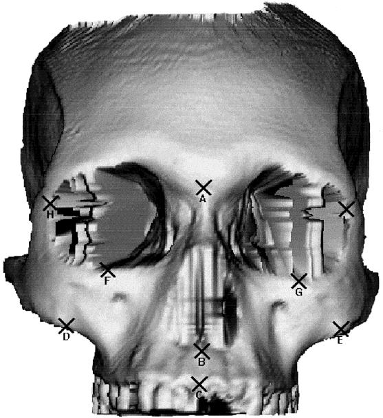
Fig 3. Landmarks shown on an Australian aborigine skull: A, nasion; B, nasospinale; C, prosthion; D, E, zygomaxillare; F, G, orbitale; H, I, frontomalare anterior.(5)
Table 5. Classification statistics for discriminant and regression analyses of paired groups.(5) |
 |
1Percentage of samples misclassified by discriminant analysis and the regression analysis. Groups 1 and 2 refer to first and second groups in pairings. |
What “ideal facial proportions” could be is addressed subsequently.
References
- Howells, W. W., Skull shapes and the map, Pap Peabody Museum Archaeol Ethnol, 79, 1 (1989).
- Roseman, C. C., Detecting interregionally diversifying natural selection on modern human cranial form by using matched molecular and morphometric data, Proc Natl Acad Sci U S A, 101, 12824 (2004).
- Wright, S., Evolution and the genetics of populations; a treatise, University of Chicago Press, Chicago, (1968).
- Roseman, C. C., and Weaver, T. D., Multivariate apportionment of global human craniometric diversity, Am J Phys Anthropol, 125, 257 (2004).
- Hennessy, R. J., and Stringer, C. B., Geometric morphometric study of the regional variation of modern human craniofacial form, Am J Phys Anthropol, 117, 37 (2002).