Feminine Beauty

Aesthetics in international beauty pageants: Part 1

Please note: Some images on this page are not work-safe.

Women participating in and often winning contemporary high profile beauty pageants mostly have unimpressive looks.  Just as the participants in the Olympics, science Nobel Prize nominees and candidates for the Field Medal are drawn from the best athletes, intellects and mathematicians, respectively, and the top prize goes to the very best among them, high profile beauty contests should be about the highest aesthetic standards and the most attractive women.

Toward this purpose it is necessary to address aesthetics in an international context.  Therefore, this section addresses whether it is possible to come up with objective criteria to compare the attractiveness of women from different [geographic] populations.  If this is possible, then these criteria should be used in beauty contests, but if this is not possible, then alternatives to the way contemporary beauty pageants are run should be considered.

Please note that whereas there are comparisons of physical appearance across populations within this section, the comparisons are not for the purpose of comparing the attractiveness of ethnic groups, but for determining whether one can come up with objective criteria to compare the attractiveness of individuals across populations.  Additionally, the illustrative examples and comparisons should not be assumed to imply typicality or average differences; the context of the illustrative examples is explained in the text and/or legends.

This section will be expanded in due time.  Comments concerning this part of the site can be left here or emailed to the author.

Section added: June 11, 2006.

Page 1 of 7 [page links: 1, 2, 3, 4, 5, 6, 7]

---

Introduction to ethnic variation: sharp contrasts and average differences

Anyone familiar with human physical variation knows that an objective comparison of attractiveness across populations must discard some traits that are known to vary greatly; e.g., skin color.  Therefore, there is an upper limit to how exacting the aesthetic criteria can be.  On the other hand, aesthetic criteria in a beauty pageant must be sufficiently exacting to separate the more attractive from the less attractive.  The question is whether one can objectively come up with aesthetic criteria to compare the attractiveness of individuals from different populations.

Some universal aesthetic criteria -- such as having blemishless and youthful skin -- are intuitive, but blemishless, youthful skin typically does not differentiate young attractive individuals from young unattractive individuals.  Since the contestants in a beauty pageant are young adults without blemishes/physical abnormalities, components of beauty related to youth and medical normality are not sufficiently discriminating to separate the more attractive from the less attractive.  Therefore, the focus here is on differences between populations and variation within the medically normal range.

Those who wanted others to believe that it is impossible to come up with objective and sufficiently exacting criteria to compare the attractiveness of individuals across populations would tend to display striking contrasts (Figures 1a-h), whereas those who wanted others to conclude the opposite would pick images that minimize differences across populations (Figures 2a-c).  Therefore, it is not sufficient to just rely on pictures to answer the central question of this section of the site.  It is necessary to also refer to average differences between populations, as documented in the anthropological literature.

 

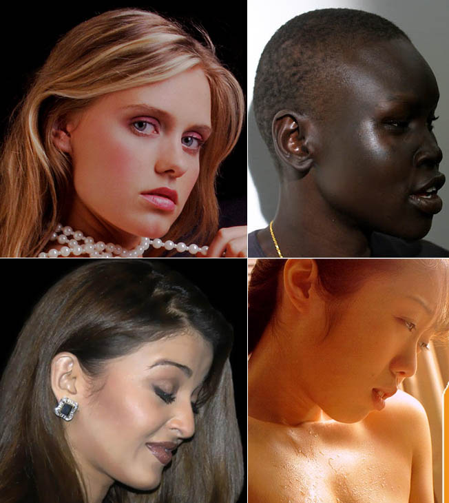
Fig 1a. Shown clockwise from top-left: European, Dinka, Japanese, Hindu.  The European is Angel from beauty is divine (adult site), the African is supermodel Alek Wek, the Japanese is glamour model Juri Hamaoka and the East Indian is Miss World 1994 Aishwarya Rai.

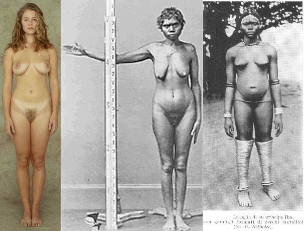
Fig 1b. Shown from left: European, Australian, Ibo.

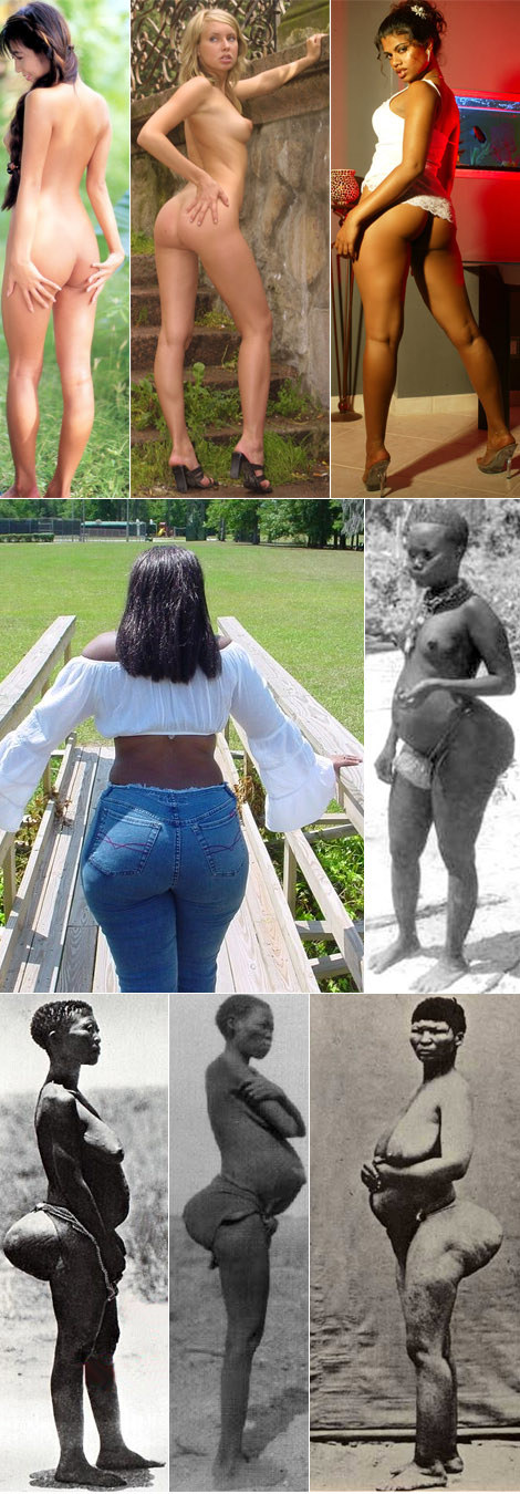
Fig 1c. Shown clockwise from top-left: Japanese, Eastern European, Bangladeshi, Andamanese, Khoikhoi, Khoikhoi, !Kung, African-American.  The Japanese is Ai Iijima, the woman from Bangladesh is Jasmyn from cinnamonbunz (adult site) and the African-American is Tropicanna from Ms. ass like whoa (adult site).

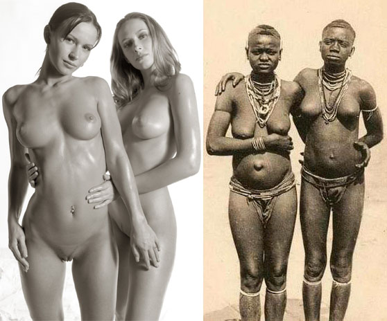
Fig 1d. Europeans and Africans.  Europeans from gallery Carré (adult site).

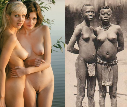
Fig 1e. Eastern Europeans (Olesia and Natasha from Met Art; adult site) and Africans.

Fig 1f. Xingu Indians, Brazil; click for larger image.

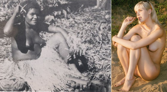
Fig 1g. Pacific Islander and Eastern European (from Met Art; adult site).

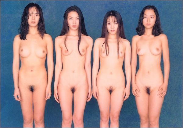
Fig 1h. Northeast Asians.

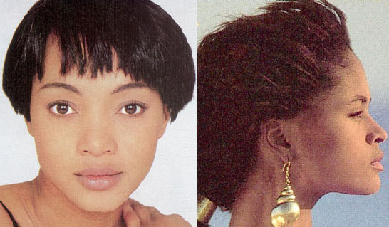
Fig 2a. Stephen Marquardt has used these two women as examples of sub-Saharan African women that illustrate the applicability of his beauty mask to attractive sub-Saharan Africans.  Marquardt’s work is addressed later on, but these women appear to have substantial European ancestry.  It would be impressive if Marquardt could show how his beauty mask applies to both Europeans and more representative examples of sub-Saharan Africans, as shown above (e.g., Fig 1a).

Fig 2b. East Asian?  No, part European and part East Asian; Leah Dizon.

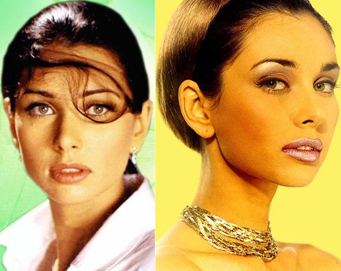
Fig 2c. Mediterranean?  No, part East Indian, part European; Lisa Ray.

To start with, the apportionment of craniofacial diversity with respect to 57 linear measurements across 10 populations from William White Howells’ dataset(1) is considered below.  The populations sampled are shown in Table 1.

Table 1. Populations studied.(2)
South America	Yauyos (110)
China	Anyang (42)
Japan	North Kyushu (91)
Siberia	Buriats (109)
Europe	Medieval Norse (110)
Middle East	Gizeh (111)
Melanesia	Tolai (83)
East Africa	Telta (83)
South Africa	!kung/San (90)
West Africa	Dogon (99)

In molecular genetics, the apportionment of genetic diversity is often described in terms of Sewall Wright’s fixation index, F_ST, which is calculated by subtracting the average diversity within populations from the total diversity in the species and then dividing the result by the total diversity in the species.  Therefore, if all the variation is within populations and none between, F_ST = 0.  If all the variation is between populations and none within, F_ST = 1.  Hence, higher F_ST values reveal greater differences between populations.  F_ST values vary depending on the locus assessed.  In animals, almost all genes are found in nuclear DNA, which is found in the nucleus of a cell.  Overall F_ST values based on nuclear DNA are classified as suggesting the following extent of genetic differentiation between populations: 0-0.05, little differentiation; 0.05-0.15, moderate differentiation; 0.15-0.25, great differentiation; 0.25-plus, very great differentiation.(3)  Overall F_ST based on nuclear DNA is about 0.15 for humans.

Roseman calculated Q_ST values for 57 linear craniofacial measurements in the 10 populations shown in Table 1, and these values are shown in Table 2.(2)  Q_ST represents the same idea as F_ST, but is designated differently to distinguish it from F_ST.  Table 2 shows that several craniofacial measurements vary very greatly across human populations.  The overall Q_ST value was 0.24, which borders on the very great.  For any given set of facial measurements, a similar proportion of people across populations will match the set if Q_ST = 0, but the problem is that Q_ST values close to zero are attained for traits such as the length of the foramen magnum (a big hole in the bottom of the skull through which the spinal cord passes), which is a trait that is not relevant to a beauty contest.  The facial measurements most relevant to a beauty contest -- such as distance between the eyes, forehead projection, nose height, jaw projection, etc. -- show very great differences across populations.     

Table 2. QST values.(2)
Measurement	QST		Full measurement name (alphabetical order)
AUB	0.49		ASB, biasterionic breadth
XCB	0.47		AUB, biauricular breadth
ZYB	0.37		AVR, molar alveolus radius
NLH	0.37		BBH, basion-bregma height
SIS	0.36		BNL, basion-nasion length
NDS	0.35		BPL, basion-prosthion length
WMH	0.34		DKB, interorbital breadth
WCB	0.32		DKR, dacryon radius
EKR	0.31		DKS, dacryon subtense
XFB	0.31		EKB, biorbital breadth
NPH	0.30		EKR, ectoconchion radius
ZOR	0.28		FMB, bifrontal breadth
SSR	0.27		FMR, frontomalare radius
VRR	0.27		FOL, foramen magnum length
FMR	0.26		FRC, nasion-bregma chord
PRR	0.25		FRF, nasion-subtense fraction
BBH	0.25		FRS, nasion-bregma subtense
ZMR	0.25		GLS, glabella projection
JUB	0.25		GOL, glabella-occipital length
ASB	0.23		IML, malar length, inferior
BPL	0.23		JUB, bijugal breadth
STB	0.23		MAB, palate breadth
DKR	0.21		MDB, mastoid width
NLB	0.21		MDH, mastoid height
NAR	0.20		MLS, malar subtense
GLS	0.20		NAR, nasion radius
SSS	0.20		NAS, nasio-frontal subtense
PAF	0.19		NDS, naso-dacryal subtense
AVR	0.19		NLB, nasal breadth
NAS	0.18		NLH, nasal height
IML	0.18		NOL, nasio-occipital length
XML	0.18		NPH, nasion-prosthion height
MAB	0.18		OBB, orbit breadth
OBH	0.16		OBH, orbital height
ZMB	0.16		OCC, l-opisthion chord
OCS	0.15		OCF, l-subtense fraction
BNL	0.15		OCS, l-opisthion subtense
EKB	0.14		PAC, bregma-lambda chord
GOL	0.14		PAF, bregma-subtense fraction
NOL	0.14		PAS, bregma-lambda subtense
DKS	0.13		PRR, prosthion radius
OBB	0.13		SIS, simotic subtense
FRS	0.13		SOS, supraorbital projection
FMB	0.13		SSR, subspinale radius
OCC	0.12		SSS, bimaxillary subtense
DKB	0.11		STB, bistephanic breadth
PAC	0.11		VRR, vertex radius
WNB	0.10		WCB, minimum cranial breadth
FRF	0.09		WMH, cheek height
SOS	0.09		WNB, simotic chord
MDH	0.08		XCB, maximum cranial breadth
MLS	0.08		XFB, maximum frontal breadth
FRC	0.08		XML, malar length, maximum
MDB	0.08		ZMB, bimaxillary breadth
PAS	0.07		ZMR, zygomaxillare radius
FOL	0.05		ZOR, zygoorbitable radius
OCF	0.04		ZYB, bizygomatic breadth

It could be pointed out that the measurements in Table 2 do not separate shape from size, but this separation is easily achieved by transforming the 57 linear measurements in Table 2 to shape variables (Mosimann shape variables), which is what Roseman and Weaver did to a more extensive set of William White Howells’ database (1,734 skulls from 6 regions; comprising of a total of 18 populations).(4)

The authors then extracted factors (principal components; PCs) underlying the covariation of the shape variables using principal components analysis (PCA).  Three shape variables -- dacryon subtense, supraorbital projection, and glabella projection -- tended to dominate the first few PCs, and were therefore excluded from PCA.  The respective variances explained by the first 8 principal components, starting from the first, were: 26.1%, 9.7%, 7.2%, 6.6%, 6.4%, 5.3%, 3.6% and 3.4%.  The first 6 PCs were most relevant and together accounted for 61.3% of the variance.  What the first six PCs correspond to is shown in Table 3 (bolded).

Table 3. Eigenvectors for first six principal components.(4)
Measurement	PC1	PC2	PC3	PC4	PC5	PC6
GOL: glabella-occipital length	-0.03	0.02	-0.04	-0.04	0.05	0.02
NOL: nasio-occipital length	-0.02	0.03	-0.05	-0.04	0.05	0.02
BNL: basion-nasion length	-0.01	0.01	-0.02	0.03	-0.01	0.05
BBH: basion-bregma height	-0.04	0.03	-0.03	-0.11	-0.01	-0.03
XCB: maximum cranial breadth	-0.03	0.04	-0.05	-0.15	0.03	-0.04
XFB: maximum frontal breadth	-0.03	0.07	-0.04	-0.16	0.00	-0.04
STB: bistephanic breadth	-0.03	0.10	-0.06	-0.20	0.02	-0.05
ZYB: bizygomatic breadth	-0.03	-0.01	0.01	-0.03	-0.01	-0.04
AUB: biauricular breadth	-0.04	0.01	-0.02	-0.06	0.00	-0.03
WCB: minimum cranial breadth	-0.04	0.01	-0.01	-0.09	0.00	-0.04
ASB: biasterionic breadth	-0.03	0.02	-0.03	-0.09	0.07	-0.02
BPC: basion-prosthion length	-0.04	0.01	0.02	0.05	-0.01	0.07
NPH: nasion-prosthion height	-0.01	-0.07	-0.03	0.00	-0.02	-0.00
NLH: nasal height	-0.00	-0.04	-0.05	-0.02	-0.03	0.00
OBH: orbital height	-0.03	0.03	-0.10	-0.08	0.02	-0.01
OBB: orbit breadth	-0.04	0.00	-0.04	-0.02	0.00	0.02
JUB: bijugal breadth	-0.03	0.02	0.03	0.00	-0.02	-0.01
NLB: nasal breadth	-0.02	0.09	0.01	0.01	-0.02	-0.00
MAB: palate breadth	-0.04	-0.03	-0.00	-0.02	-0.01	-0.00
MDH: mastoid height	0.02	-0.28	0.19	0.05	0.08	-0.48
MDB: mastoid width	-0.02	-0.36	0.35	0.10	0.19	-0.42
ZMB: bimaxillary breadth	-0.03	0.02	0.01	0.01	-0.01	-0.05
SSS: bimaxillary subtense	-0.01	-0.16	-0.42	0.16	-0.11	-0.02
FMB: bifrontal breadth	-0.03	0.03	-0.01	0.01	-0.01	-0.01
NAS: nasio-frontal subtense	0.10	-0.01	-0.30	0.53	-0.09	0.03
EKB: biorbital breadth	-0.03	0.04	0.00	-0.00	-0.00	-0.00
DKB: interorbital breadth	0.00	0.20	0.04	0.18	-0.00	-0.06
NDS: naso-dacryal subtense	0.18	-0.19	-0.16	0.14	-0.09	0.05
WNB: simotic chord	0.54	0.66	0.18	0.19	0.12	-0.24
SIS: simotic subtense	0.77	-0.36	-0.02	-0.36	-0.06	0.21
IML: malar length, inferior	-0.03	0.01	0.26	0.10	-0.09	0.19
XML: malar length, maximum	-0.03	-0.02	0.17	0.06	-0.06	0.13
MLS: malar subtense	-0.07	-0.00	0.55	-0.01	-0.08	0.43
WMH: cheek height	-0.01	-0.07	0.17	0.03	-0.01	-0.07
FOL: foramen magnum length	-0.04	0.01	-0.07	-0.05	-0.03	0.04
FRC: nasion-bregma chord	-0.04	0.04	-0.05	-0.11	0.03	0.00
FRS: nasion-bregma subtense	-0.07	0.22	-0.14	-0.32	0.10	0.09
FRF: nasion-subtense fraction	-0.05	-0.04	-0.01	-0.06	-0.03	-0.00
PAC: bregma-lambda chord	-0.04	0.07	-0.03	-0.13	-0.12	-0.09
PAS: bregma-lambda subtense	-0.07	0.12	0.02	-0.28	-0.49	-0.29
PAF: bregma-subtense fraction	-0.03	0.09	-0.02	-0.14	-0.16	-0.12
OCC: lambda-opisthion chord	-0.04	0.02	-0.06	-0.11	0.21	0.01
OCS: lambda-opisthion subtense	-0.03	0.02	-0.09	-0.01	0.58	0.13
OCF: lambda-subtense fraction	-0.04	-0.02	-0.05	-0.15	0.44	-0.04
VRR: vertex radius	-0.04	0.04	-0.03	-0.15	0.00	-0.06
NAR: nasion radius	-0.01	0.02	-0.03	0.05	-0.02	0.06
SSR: subspinale radius	-0.03	-0.01	-0.03	0.07	-0.04	0.08
PRR: prosthion radius	-0.04	-0.00	-0.01	0.06	-0.03	0.08
DKR: dacryon radius	-0.03	0.04	-0.02	0.04	-0.01	0.08
ZOR: zygoorbitable radius	-0.04	0.03	0.03	0.05	-0.02	0.10
FMR: frontomalare radius	-0.04	0.03	0.03	-0.05	-0.00	0.08
EKR: ectoconchion radius	-0.05	0.03	0.05	-0.03	-0.01	0.09
ZMR: zygomaxillare radius	-0.05	0.04	0.10	0.04	-0.02	0.13
AVR: molar alveolus radius	-0.04	-0.02	0.02	0.08	-0.02	0.09
* Coefficients with an absolute value > 0.2 are in bold.

The Q_ST values for the shape PCs are shown in Table 4.

Table 4. Proportion of variance found between regions.(4)
Variable	QST
Shape PC1	0.24
Shape PC2	0.33
Shape PC3	0.08
Shape PC4	0.19
Shape PC5	0.07
Shape PC6	0.04
Size (log geometric mean)	0.22
All 54 shape PCs	0.15
6 retained shape PCs	0.17
15 retained shape PCs	0.17
Shape PCs 7–54	0.14
Shape PCs 16–54	0.14

Once again, a number of great and very great differences in shape are seen, and the largest of these, involving PC1 and PC2, cluster in the upper nasal region, which is important in a beauty contest. 

Therefore, for any given set of “ideal facial measurements,” the proportion of people from different geographic populations that will match the set of measurements will vary greatly.  An idea of the great variability of this statistic across populations can be appreciated by noting that even a small number of facial measurements (Fig 3) largely distinguish geographic populations (Table 5), but in a beauty contest, a large number of facial measures need to be evaluated.

Fig 3. Landmarks shown on an Australian aborigine skull: A, nasion; B, nasospinale; C, prosthion; D, E, zygomaxillare; F, G, orbitale; H, I, frontomalare anterior.(5)

Table 5. Classification statistics for discriminant and regression analyses of paired groups.(5)

1Percentage of samples misclassified by discriminant analysis and the regression analysis.  Groups 1 and 2 refer to first and second groups in pairings.

 What “ideal facial proportions” could be is addressed subsequently.

References   

1. Howells, W. W., Skull shapes and the map, Pap Peabody Museum Archaeol Ethnol, 79, 1 (1989).
2. Roseman, C. C., Detecting interregionally diversifying natural selection on modern human cranial form by using matched molecular and morphometric data, Proc Natl Acad Sci U S A, 101, 12824 (2004).
3. Wright, S., Evolution and the genetics of populations; a treatise, University of Chicago Press, Chicago, (1968).
4. Roseman, C. C., and Weaver, T. D., Multivariate apportionment of global human craniometric diversity, Am J Phys Anthropol, 125, 257 (2004).
5. Hennessy, R. J., and Stringer, C. B., Geometric morphometric study of the regional variation of modern human craniofacial form, Am J Phys Anthropol, 117, 37 (2002).

---

Page 1 of 7 [page links: 1, 2, 3, 4, 5, 6, 7]