The previous entry on the Marquardt Phi (golden ratio) mask application pointed out that Marquardt’s methodology doesn’t adjust for size before comparing shape. We now consider how to adjust for size as well as other standardization procedures prior to comparing shape.
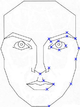
A shape can be roughly represented in terms of its landmarks, an example of which is shown in Fig. 1 (the crosses mark the landmark points). If Fig. 1 were just shown as dots where the crosses are, and nothing else, one could connect the dots to get a face that resembles Marquardt’s mask, and it would have important proportions the same as in Marquardt’s mask. If one had a bunch of faces to compare, then one could measure the positions of corresponding landmarks for each of the faces in terms of the x- and y-coordinate of each landmark, and proceed as follows.
Fig. 1. Landmarks identified by crosses on the outline of the Marquardt golden ratio mask. Landmarks are shown for one side of the face; both sides of the face are assessed.
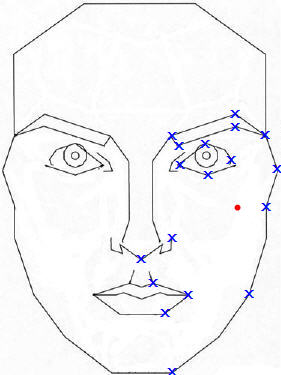
Consider the red dot in Fig. 2. One can compute the magnitude of the average distance between the red dot and all other landmarks. If the red dot were moved around, this average distance will change. Our interest is the position of the red dot that corresponds to the least magnitude of the average distance between it and the landmarks; call this position the centroid. If the same amount of mass were placed at each landmark of the shape, then the centroid would be the point around which the mass is equally distributed, i.e., the system’s center of mass.
Technical: The centroid of a system is the position corresponding to the least sum of squared distances between it and the landmarks of the system.
Fig 2. The red dot can be moved so that the sum of squared distances between it and the landmarks is minimized; landmarks shown for only one side of the face.
The magnitude of the average distance between the centroid and the landmarks will increase with the size of the object. Call this average distance the centroid size.
Technical: The centroid size of a system is the sum of squared distances between the centroid and the system’s landmarks.
So how does one adjust for size before comparing shape? One simply adjusts for the centroid size. For instance, if one face has a centroid size of 42 units and another of 53 units, then the second face can be scaled down so that it, too, has a centroid size of 42 units. One is not limited to choosing either 42 or 53 in this case. Both images can be scaled to, say, a centroid size of 24 units. Usually, the shapes to be compared are scaled to a centroid size of 1.
So the size issue is taken care of, but before superimposing one image on another to compare shape, like Marquardt does, how does one align them? One simply aligns them at the centroid. There is yet another issue. Each image can be rotated around its centroid. So what rotational positions does one assign to the images before they are superimposed/compared? One rotates the images so that the magnitude of the average distance between corresponding landmarks is minimized.
Technical: The rotation serves to minimize the sum of squared distances between corresponding landmarks.
And that is it; now one can compare shape. So before one compares shapes, the following procedures are performed.
- Assign landmarks.
- Measure the coordinates of corresponding landmarks on all figures.
- Scale all figures to the same centroid size.
- Align the figures at their centroids.
- Rotate the figures so that the sum of squared distances between corresponding landmarks in minimized.
This procedure is known as Procrustes analysis, a standard technique in physical anthropology. For more on shape analysis, see a paper by O’Higgins,(1, pdf) and the more math-oriented can look up a paper by Fred Bookstein.(2, pdf)
Sometimes it can be difficult to locate corresponding landmarks (Fig. 3). In such cases, one is dealing with semi-landmarks or sliding landmarks, not true landmarks. There is a way to deal with sliding landmarks,(3, pdf) but people who simply wish to see how Procrustes analysis works can choose sufficiently different faces and use a simple approximation: the y-coordinate (vertical axis coordinate in Fig. 3) of the sliding landmark is the point of intersection of straight lines most closely approximating Marquardt’s mask’s jaw outline, and the x-coordinate is obviously the position at which the jawline has this y-coordinate.
Fig. 3. The landmarks on the jawline of the Marquardt mask are easy to place, but not so easy in the case of the right image.
Naturally, nobody would do the calculations by hand. All one needs to do is to measure the coordinates (landmark positions for each shape) and a computer will do the rest. There are a number of image editing/processing programs that provide the coordinates of a point if you hold the cursor above it. For all images, note down the x- and y-coordinates of each landmark, and write them down in the same order. For instance, if the order is “left outer eye corner, left inner eye corner, right inner eye corner,” then write down the coordinates in this order for each face. If the corresponding coordinates for these measurements are (120, 500), (150, 495), (178, 496), then for the statistical package mentioned below, simply list them in a text file (.txt) -- each face’s coordinates are listed on a separate text file -- as
120 500 150 495 178 496
You could write the above as...
120 500
150 495
178 496
...and it wouldn’t make any difference. The important points are at least a single gap between each listing and entering the landmark measurements in the same order for all faces. Measure the coordinates for each face twice. The second set of measurements is entered in the text file after the first set:
Set 1 measurements
Set 2 measurements
Let us compare two faces, face A and face B. Their corresponding measurements are in the text files facea.txt and faceb.txt, respectively.
An open source software environment that can be used for shape analysis is R. After installing R, start the program and install the shapes package(4) as follows:
Go to the top menu > select packages > install package(s) > select mirror (closest country/location) > select “shapes” -- system will download and install it.
Load the shapes package by typing the following and clicking enter/return:
library(shapes)
Let k be the number of landmarks and m the number of dimensions (the images shown above have two dimensions, x and y axes)
Let us say you have 11 landmarks and 2 dimensions; load the face data as follows:
k<-11
m<-2
facea.dat<-read.in("c:/facea.txt",k,m)k<-11
m<-2
faceb.dat<-read.in("c:/faceb.txt",k,m)
In the examples above, the txt files are in the C:/ directory. Adjust path to location if the location is different.
The distance between faces A and B can be calculated as follows:
facea<-procGPA(facea.dat)
faceb<-procGPA(faceb.dat)
rho<-riemdist(facea$mshape,faceb$mshape)
cat("Riemannian distance between mean shapes is ",rho," \n" )
This will return a value between 0 and π/2; the closer to zero, the smaller the shape difference between the faces. Note that Marquardt’s method doesn’t allow one to provide a quantitative estimate of how close two shapes are, but after Procrustes analysis, one can describe the Riemannian distance between two shapes/two sets of shapes.
To visualize the nature of shape differences, use thin plate splines analysis. Enter the following:
#TPS grid with shape change exaggerated (1x)
facea<-procGPA(facea.dat)
faceb<-procGPA(faceb.dat)
mag<-1
TT<-facea$mshape
YY<-faceb$mshape
par(mfrow=c(1,2))
YY<-TT+(YY-TT)*mag
tpsgrid(TT,YY,-0.6,-0.6,1.2,2,0.1,22)
title("TPS grid: facea (left) to faceb (right)" )
The magnification factor helps one visualize subtle changes by exaggerating the shape difference by a specified factor. In the example above, the magnification factor is simply 1 (mag<-1; no exaggeration). To exaggerate the shape difference three-fold, use mag<-3. The other numbers can be left as they are; what they mean can be read about in the manual for the shapes package for R. The manual describes other things one can do with shape analysis.
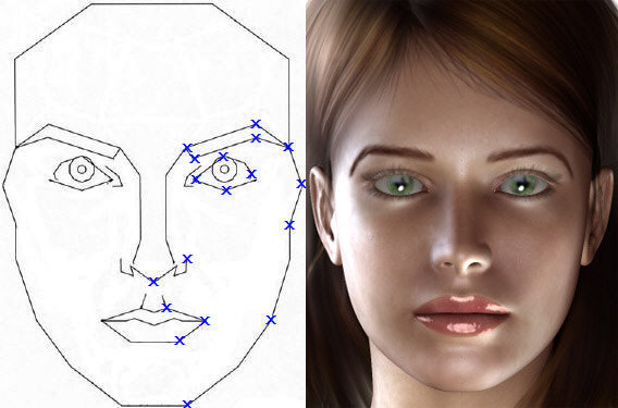
A sample output of the thin plate splines analysis is shown in Fig. 4. The deformation of the two-dimensional grid in the background shows how the sample faces differ from Marquardt’s mask.
Fig. 4. Thin plate splines. The human pictures are from Marquardt's site. The deformation of the 2-D grid shows how the human faces differ from Marquardt's mask's shape.
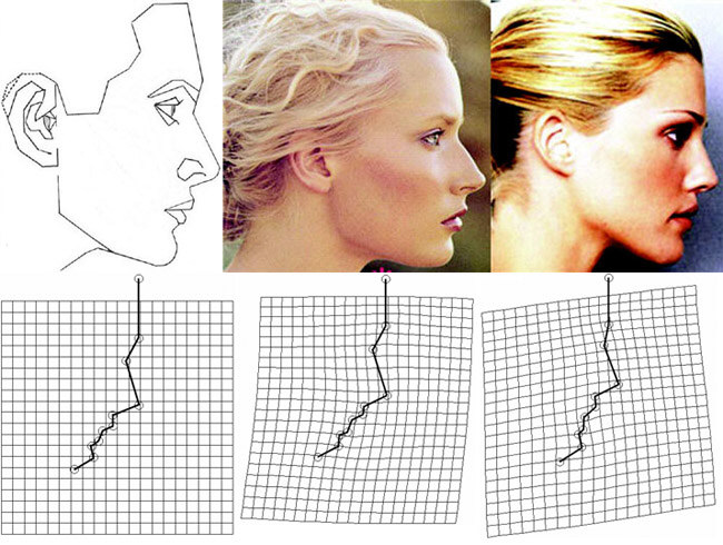
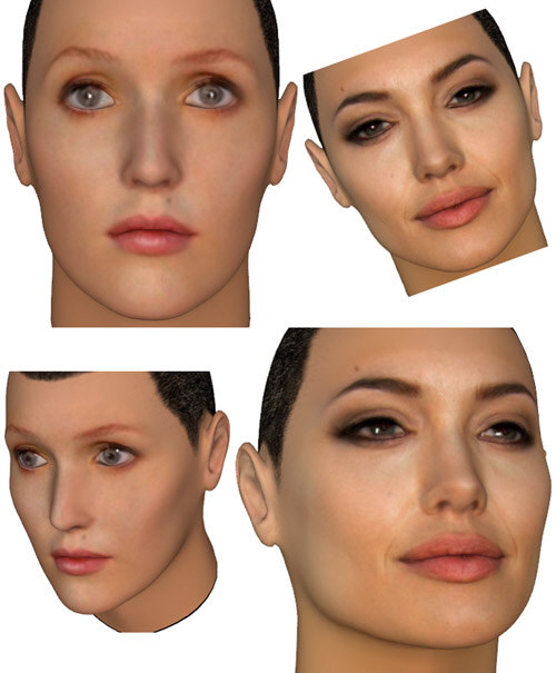
Since the Procrustes analysis algorithm adjusts for size and rotational effects, even if the shapes being compared have their landmark coordinates measured under different sizes and rotational positions as in the first row of Fig. 5. it will make no difference as long as the measurements are entered in the same order. However, since the measurements are in two dimensions, x and y, recording measurements as in the second row of Fig. 5 will be invalid because the images are being rotated in a third dimension that is not being controlled for. On the other hand, if the shape comparison were in three dimensions, then measuring the coordinates as in the second row of Fig. 5 would be valid.
Fig. 5. 3-D art by Strigoi, depicting Gillian Anderson (left) and Angelina Jolie. In practice (actual measurements), both faces will have the same neutral expression. See text for context.
The most convenient way of assessing face shapes in three dimensions is to use a laser scanner. If one wanted smooth outputs, then instead of the hassle of dealing with a huge number of landmarks, one can use techniques that impute the positions of points (pseudo-landmarks) between landmarks.(5, pdf)
I will come up with some illustrations of face shape comparisons in reference to Marquardt’s mask later.
References
- O'Higgins, P., The study of morphological variation in the hominid fossil record: biology, landmarks and geometry, J Anat, 197, 103 (2000).
- Bookstein, F. L., Biometrics, biomathematics and the morphometric synthesis, Bull Math Biol, 58, 313 (1996).
- Bookstein, F. L., Landmark methods for forms without landmarks: morphometrics of group differences in outline shape, Med Image Anal, 1, 225 (1996/7).
- Dryden, I. L., and Mardia, K. V., Statistical Shape Analysis, John Wiley, Chichester (1998).
- Hutton, T. J., Buxton, B. F., Hammond, P., and Potts, H. W., Estimating average growth trajectories in shape-space using kernel smoothing, IEEE Trans Med Imaging, 22, 747 (2003).
Comments
I've always found Gillian Anderson attractive. Her eyes are especially attractive, and they're also appropriately distanced (not too close; not too far). Her complexion creamy and freckly, indicative of youth. Despite its capacious height, her forehead is also very smooth and tall and is proportional to the rest of her face. The gonial angles on her jawline are also somewhat soft in spite of her bulging chin.
However, Gillian does have some serious flaws. Her redeeming feminine facial features are counterbalanced by her contrasting masculine features. There is first the issue of her very bulging chin, giving her a longer face that could look horse-like. The horse-like features are compounded by her cartoonishly gummy smile and masculine cheekbones (of course, the positive feature seem to balance this out far better than someone like Sarah Jessica Parker). Furthermore, she has a very long, projecting nose and a slightly pronounced nasion which has only worsened with age. Although tragically flawed by very unfeminine features, she still has a somewhat feminine face.
Then, there's the trouble with her shape. As far as Gillian's body is concerned, she has a very barrel-like physique and flat buttocks. Although she may be physically fit, her broad shoulders appear look too masculine for a woman her stature. Furthermore, she has a very narrow pelvis, a broad rib cage, and an insufficiently narrow waist. Her sagging breasts, even at the age of 23, do her no favors, either.
Richard, Gillian has not aged well at all, and her feminine features deteriorated and her masculine features augmented. Her features were already unfeminine even as a child (albeit she still had some femininity as you mentioned). Just have a look at this collage of Gillian with pictures throughout her childhood:
![]() http://23.imagebam.com/download/fFsd4KxIFgnkFZ_np8iz4g/10505/105041221/ABC.jpg
http://23.imagebam.com/download/fFsd4KxIFgnkFZ_np8iz4g/10505/105041221/ABC.jpg
![]() http://24.media.tumblr.com/tumblr_m4ugfd3ngT1rpuubxo3_400.jpg
http://24.media.tumblr.com/tumblr_m4ugfd3ngT1rpuubxo3_400.jpg
![]() http://www.gilliananderson.ws/spring/images/turning1.jpg
http://www.gilliananderson.ws/spring/images/turning1.jpg
![]() http://www.gilliananderson.ws/spring/images/turning3.jpg
http://www.gilliananderson.ws/spring/images/turning3.jpg
And here's a very unflattering photo from one of her first films:
Perhaps she's angle-dependent, as her features look much more rounded here:
If you notice, Gillian also has asymmetric eyes.
Also, Gillian has a very defined frontal bone jutting in the forehead much like Brooke Shields.